
Software Design
State Machine
The software dictating the behavior of the robot was split into two levels - a series of functions that each performed a simple action with a main structure controlling the transition between states of the mission.
Several functions controlled the components to perform specific actions such as driving forward, turning left, or launching projectiles. These functions commanded the motors and servos appropriately, using PWM to modulate the two motors’ speeds and to change the servo’s position. A PD controller was implemented for the driving functions, the feedback was provided by encoders. This controller allowed for variation in the performance of the two motors, causing the robot to travel straight when going forward and backward, and rotate in place when turning.
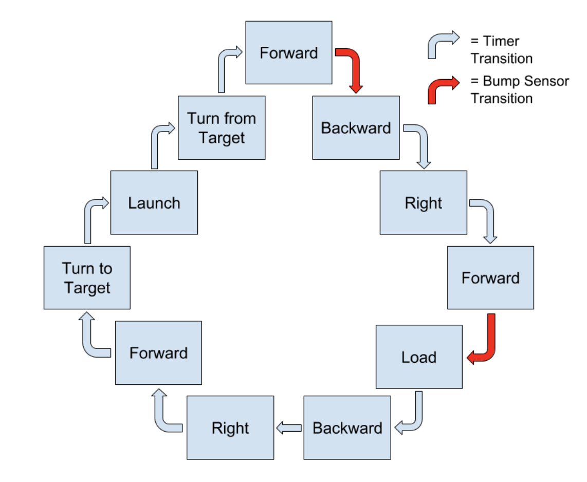
The transition between states was controlled by timers or by input from the bump sensor. For example, the robot would call the “travel forward” function during state one and the state would transition to state two when the bump sensor was triggered. During the transition to state two, the initial time was recorded, then the onboard clock was queried so that state two would end after a prescribed time. As the “travel backward” function was called during state two, the result of these two states occurring was travelling forward until hitting the wall, then moving a set distance back from the wall. This type of procedure was then continued for each step of the mission, such as setting timers to turn right 90° or turning the motors off for a prescribed time to allow for loading the robot. This methodology required tedious testing to determine the correct lengths of time required for each step, for example 650 milliseconds for a 90° turn. This tedium was required however, as the encoders did not have sufficient resolution to allow for direct control. The encoders registered 12 counts per revolution, which resulted in about 10° deviation in the orientation of the robot, deviation too great for mission success.
The state transitions are outlined in the Figure below. An important note is that turning toward and away from the target is dependent on which target is selected, which is a variable that cycles through from one to four. The times associated with each transition are repeated when possible, such as consistent times to turn 90° to the right or to move a set distance back from the wall. The robot starts in the “forward” state at the top of the diagram.
The main challenge with the method of dead reckoning is accumulation of error and the system not behaving consistently. In our case, wall riding allowed for variations to be eased out of the system. Suppose there was a 3° error when rotating to face the loading zone, so the robot was not aligned perfectly with the playing field. When driving forward and hitting the wall, the force of impact would cause the robot to twist in place such that the body is now orthogonal to the playing field. This is also why using a bump sensor was so important - it allowed for translational error to be reduced, as traveling until hitting the wall is a consistent milestone.